Seems good, so far.

Table of Contents

1. Lec 1 What is it about.
   1. I. Basic physical exapmles
   2. II. Differential equations arise from physics
      1. 1. Pendulum(downward position, with friction)
      2. 2. Pendulum(upright position, with friction)
      3. 3. LR-circuit
      4. 4. DC motor
      5. 5. Cart|with(out) friction
   3. III. Inputs and Outputs
   4. IV. Feedback
      1. 1. Our goals
2. Lec 2 Linear differential equations and their solutions
   1. I. Mathematical background
      1. 1. Solution for homogeneous linear ordinary differential equations with constant coefficients
         1. Step1 Characteristic Equation
         2. Step 2 Find algebraic roots
         3. Step 3 Find corresponding Modes
         4. Step 4 Obtain a general solution as a linear combinition of modes with unkown coefficients
         5. Step 5 Obtain the particular solution from the given initial conditions
      2. 2. Stability of modes
   2. II. Stability of a linear system
      1. 1. Definition
      2. 2. Examples
         1. a. Pendulum downwards without friction
         2. b. Pendulum downwards with friction
         3. c. Pendulum upwards
         4. d. Repeated roots
   3. III. Hurwitz criterion
      1. 1. Explanation
      2. 2. Simple corollaries
3. IV. Basic of controller design
   1. 1. No control
   2. 2. P-Controller
   3. 3. PD-Controller
      1. a. Type one
      2. b. Type two
      3. c. Check

---

Lec 1 What is it about.

---

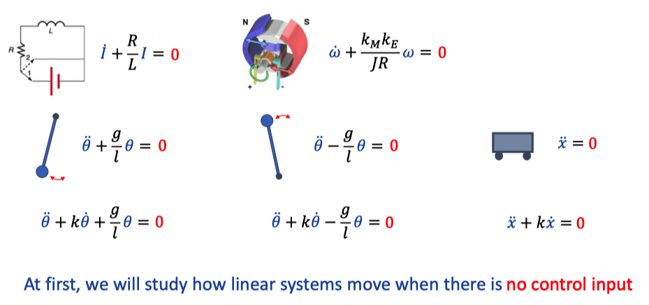
I. Basic physical exapmles

Simple Pendulum
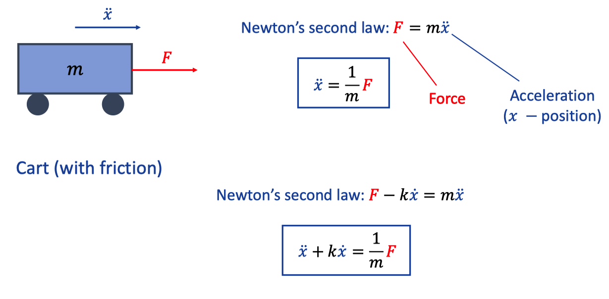
Simple Cart
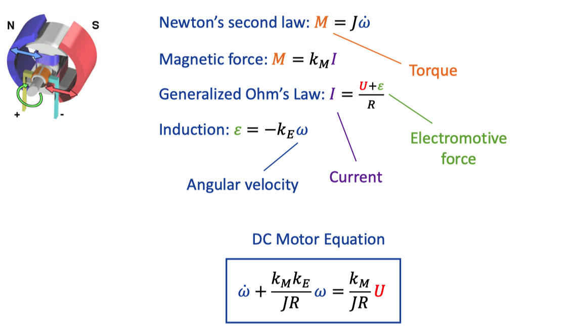
DC Motor
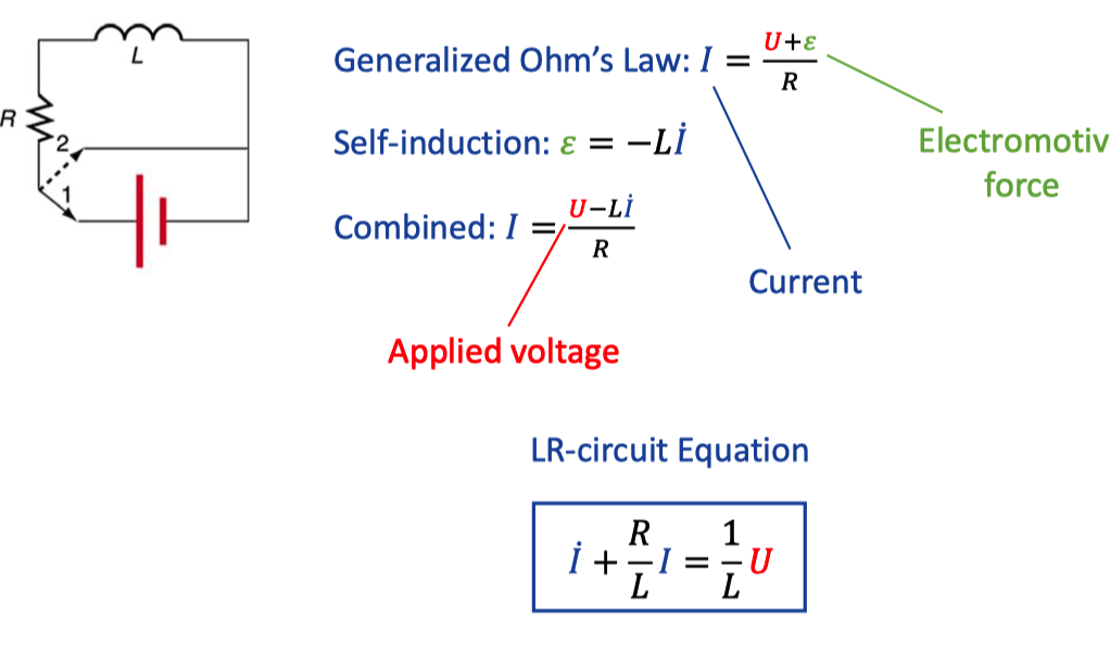
LR-Circuit(with intention, it becomes LCS)
Solar system(a little over simplified, dynamic, nonlinear)

II. Differential equations arise from physics

1. Pendulum(downward position, with friction)

Harmonic form(left), for small angle makes it linearized. Mass is concentrated on one end.

What if the friction doesn’t exist?

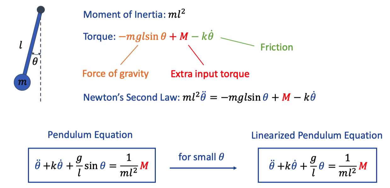
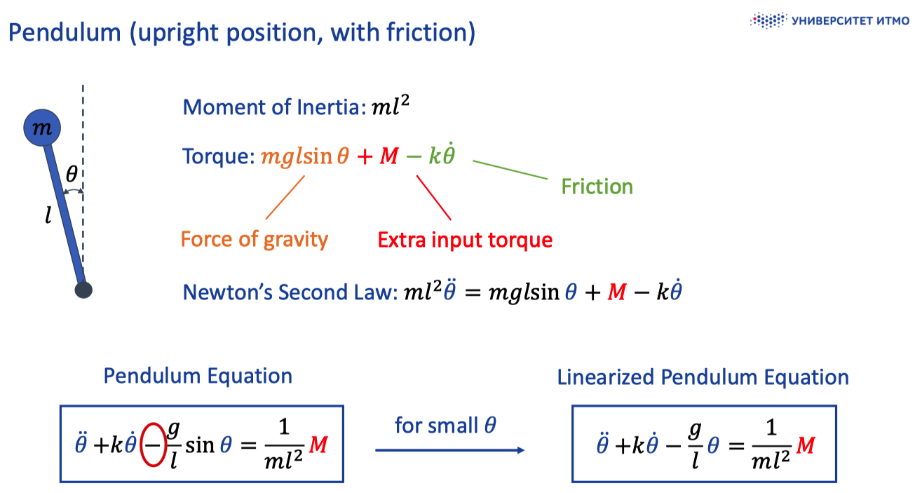
2. Pendulum(upright position, with friction)

Basically the same. Note that the equation stays true in the condition of small θ.

3. LR-circuit

Magnetic flux is L * I, electromotive force is derived from Faraday law.

4. DC motor

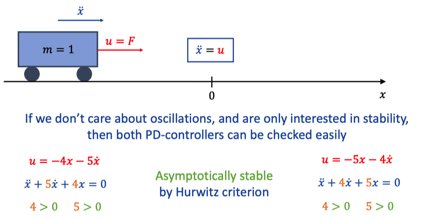
5. Cart|with(out) friction

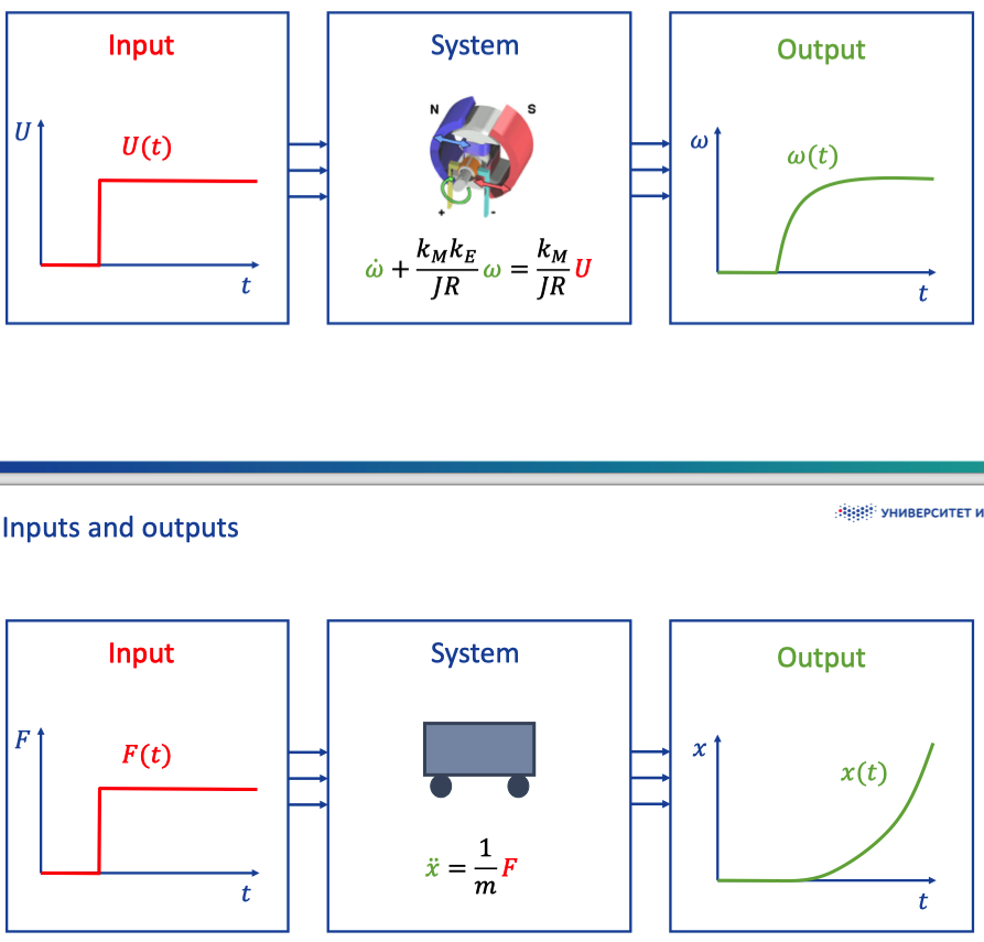
Comparing these equations, systems have inputs and outputs

III. Inputs and Outputs

Derivatives in equation makes the the speed of outputs changes.

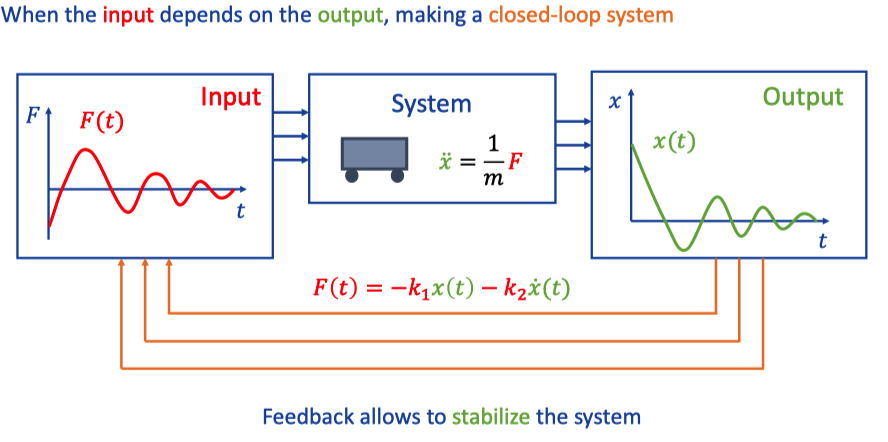
IV. Feedback

1. Our goals

Study how linear system behave on their own, without any input.

Study how linear system respond to different inputs.

Learn to design feedback controllers and state observers

Lec 2 Linear differential equations and their solutions

---

At first, we will study how linear systems move when there is no control input.

These systems can be called as autonomous systems.

In mathematics, an autonomous system or *autonomous differential equation is a system of ordinary differential equations which does not explicitly depend on the independent variable. When the variable is time, they are also called time-invariant systems.

I. Mathematical background

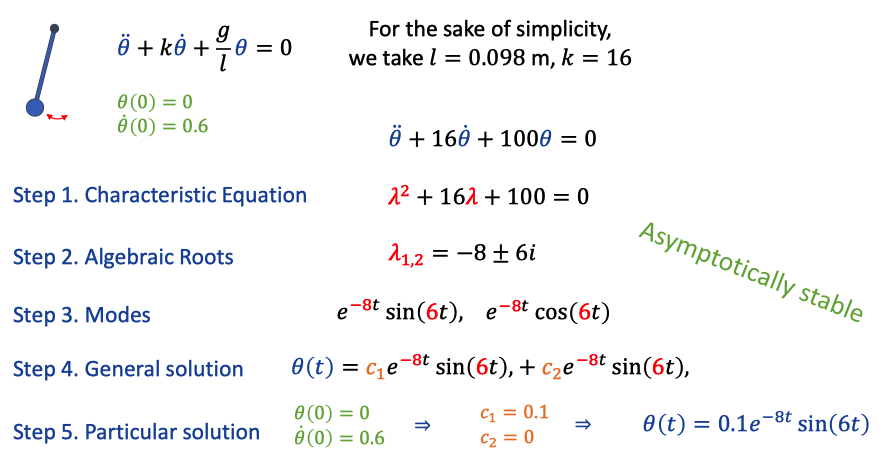
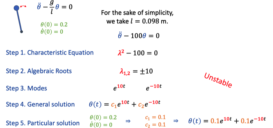
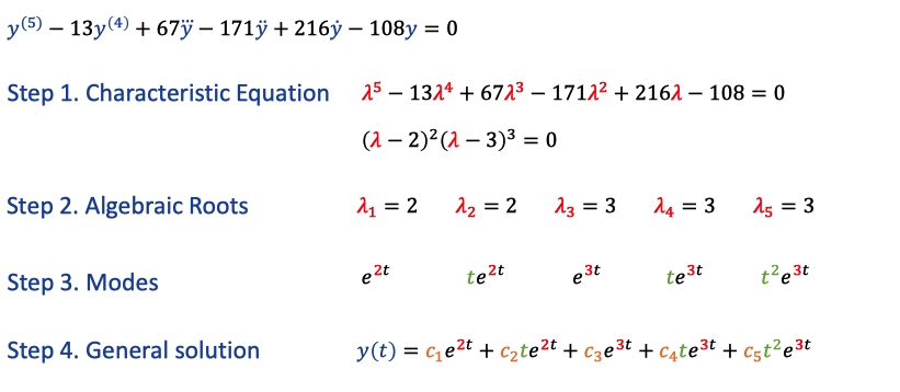
1. Solution for homogeneous linear ordinary differential equations with constant coefficients

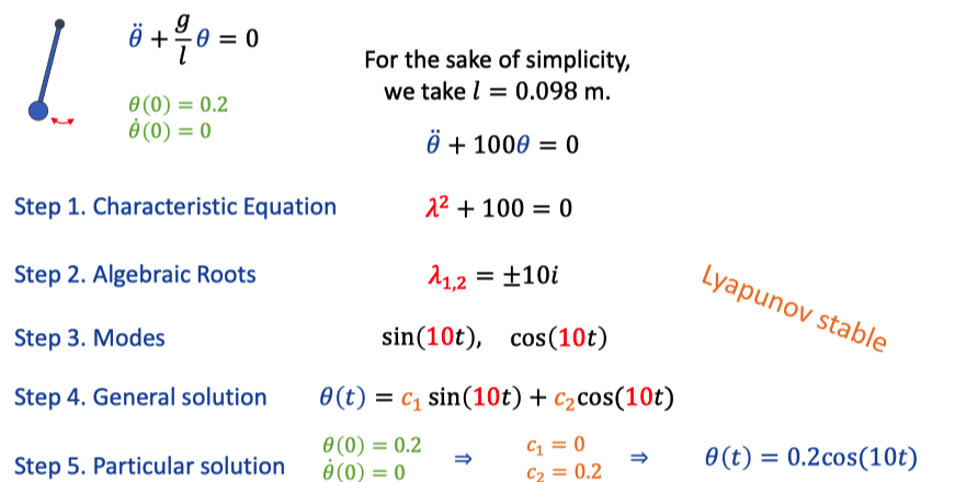
Step1 Characteristic Equation

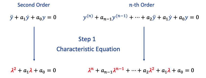
Simply rewrite the eq into algebraic eq. It doesn’t lose information.

Step 2 Find algebraic roots

Step 3 Find corresponding Modes

*Modes are simple functions from which solutions of a differential equation are combined. Linearly independent.

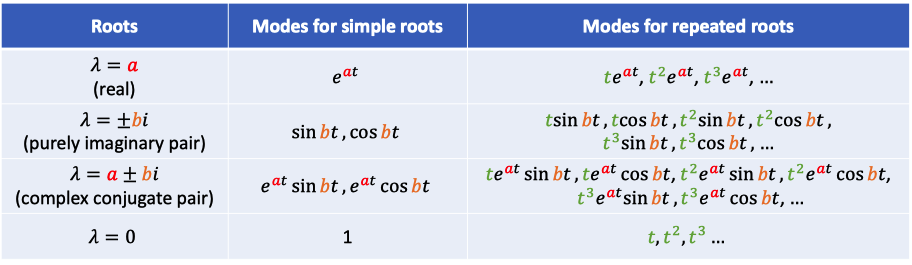
Each next multiplicity of root give you next (set of) mode multiplied by t.

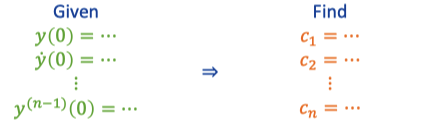
Step 4 Obtain a general solution as a linear combinition of modes with unkown coefficients

Step 5 Obtain the particular solution from the given initial conditions

2. Stability of modes

Two different situations.

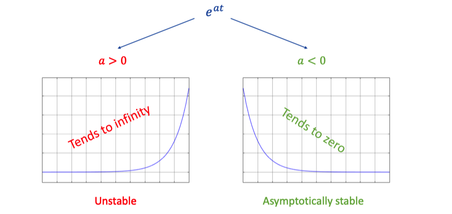
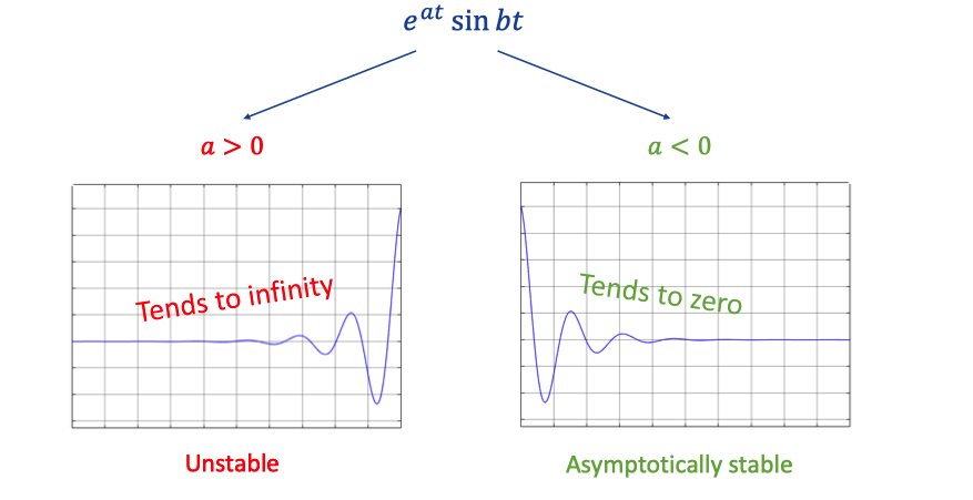
• Asymptotically is similar to gradually,, but have a tendency to a straight line.

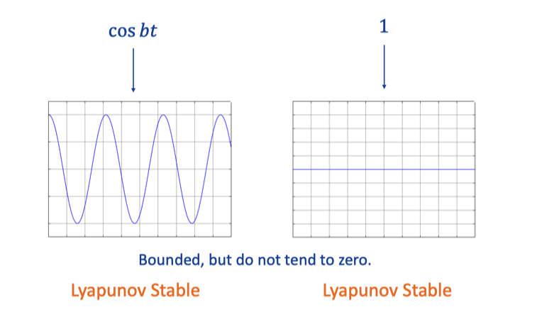
• Lyapunov - do not tend to zero.

II. Stability of a linear system

1. Definition

Linear system is asymptotically stable if all roots of characteristic equations have negative real parts. It means that y(t) tends to 0 for all initial conditions.

• Which means that you can start the system with big initial values, and it will stop.

Linear system is Lyapunov stable if all roots of characteristic equations have either negative or zero real parts, and roots that gave zero real parts are simple (not repeated). It means taht y(t) is bounded for all initial conditions.

• It’s a weaker stability, all asymptotically stable is Lyapunov stable (negative real part), but the latter (zero real parts) may not be the former.

Linear system is unable otherwise. It means taht y(t) is unbounded for some initial conditions.

2. Examples

a. Pendulum downwards without friction

b. Pendulum downwards with friction

c. Pendulum upwards

d. Repeated roots

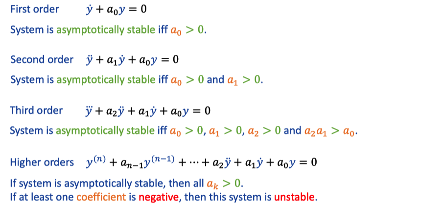
III. Hurwitz criterion

How can we check that a given system is stable or unstable without calculating roots of its characteristic equation.

1. Explanation

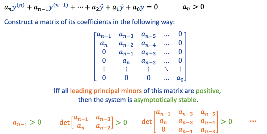
2. Simple corollaries

They could have oscillations, or not.

IV. Basic of controller design

1. No control

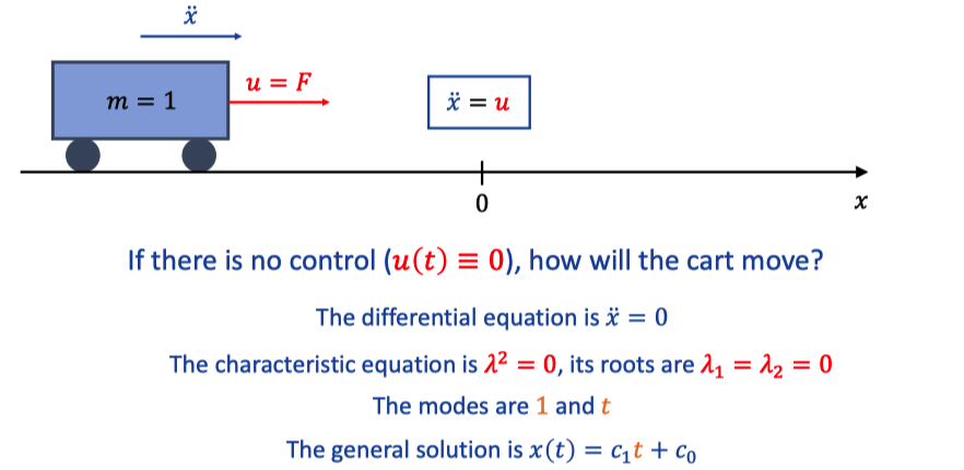
It will move in one direction with constant speed.

2. P-Controller

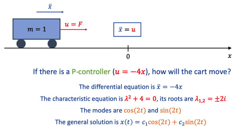
The cart oscillates around x=0 with constant amplitude.

3. PD-Controller

a. Type one

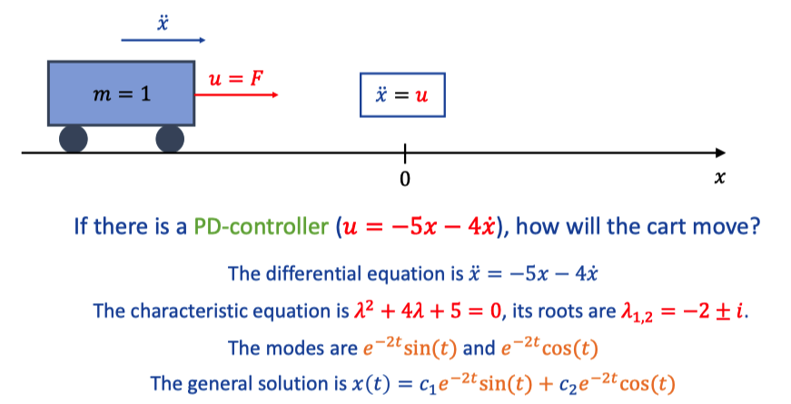
The cart oscillates around x=0 with decaying amplitide.

b. Type two

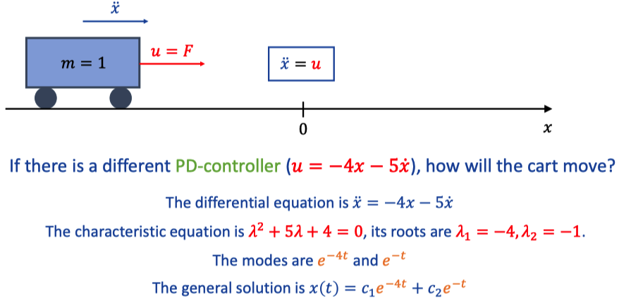
The cart slides to x=0 without oscillations.

c. Check