Should be the last one

Table of Contents

1. Lec 8 Linear feedback controllers, s.s. observers
   1. I. Lyapunov method
      1. a. Properties
      2. b. Lyapunov Theorem
      3. c. Example
   2. II. State Feedback design
      1. a. Scenary
      2. b. Example
      3. c. MATLAB realization
      4. d. Modal Control
      5. e. Example
      6. f. Observer Design
      7. g. Example
      8. h. MATLAB realization
   3. III. Combinition

Lec 8 Linear feedback controllers, s.s. observers

I. Lyapunov method

a. Properties

Let us consider Lyapunov functions for investigation stability of linear systems. Lyapunov functions have the next properties:

• Lyapunov function V (𝑥) must be positive definite: for any 𝑥 ∈ 𝑅𝑛
• Lyapunov function V (𝑥) is positive definite and V (𝑥) = 0 in case 𝑥 is null-vector (zero).
• Lyapunov functions must increases (decreases) uniformly with uniform increasing (decreasing) of 𝑥-vector norm.

That is, $\lim_{x\to 0}V(x)=0$ and $\lim_{x\to \infty}V(x)=\infty$

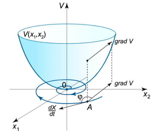
b. Lyapunov Theorem

The equilibrium 𝑥 = 0 is asymptotic stable if exists Lyapunov function V (𝑥) such that for any motion trajectories 𝑥(𝑡) starting from the arbitrary initial conditions for any time ∀𝑡 ≥ 0 the derivative of the function is negative: $\frac{dV(x(t))}{dt} < 0$.

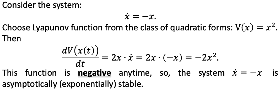
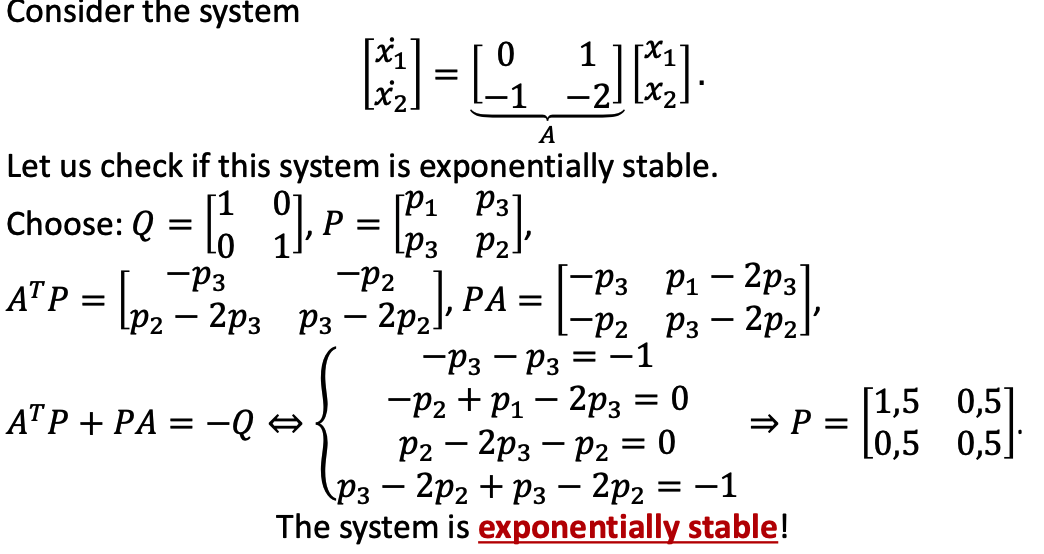
c. Example

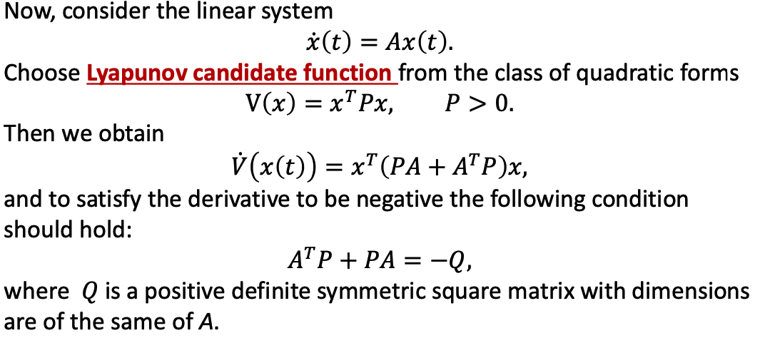
• P is symmetrical positive definite matrix. Its dimension is the same with A.
• In linear algebra, a symmetric nxn real matrix) Mis said to be positive-definite

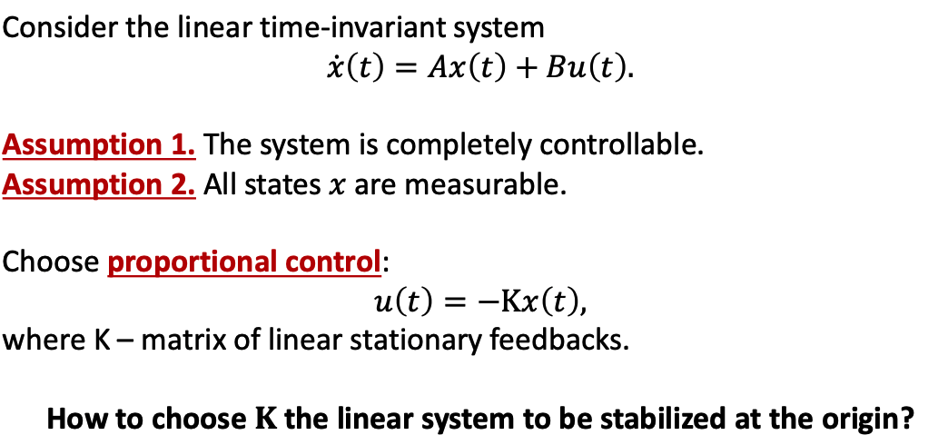
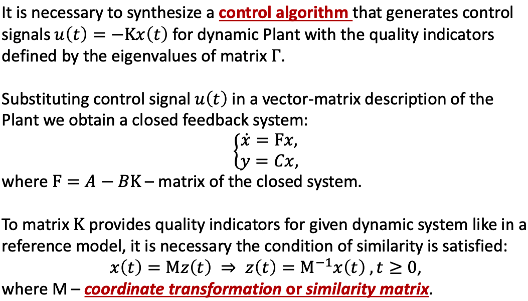
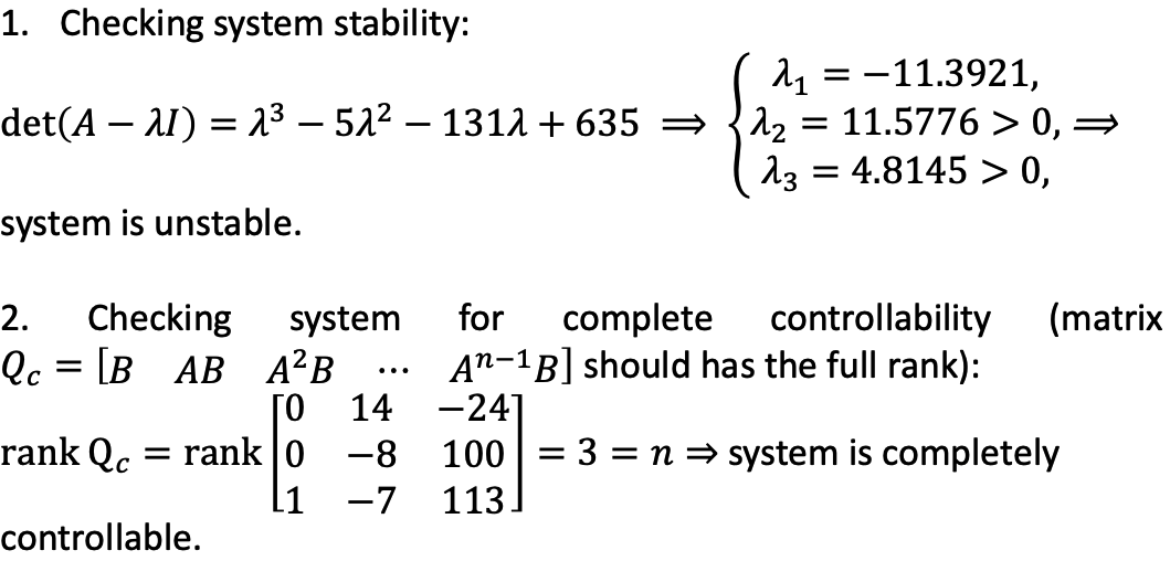
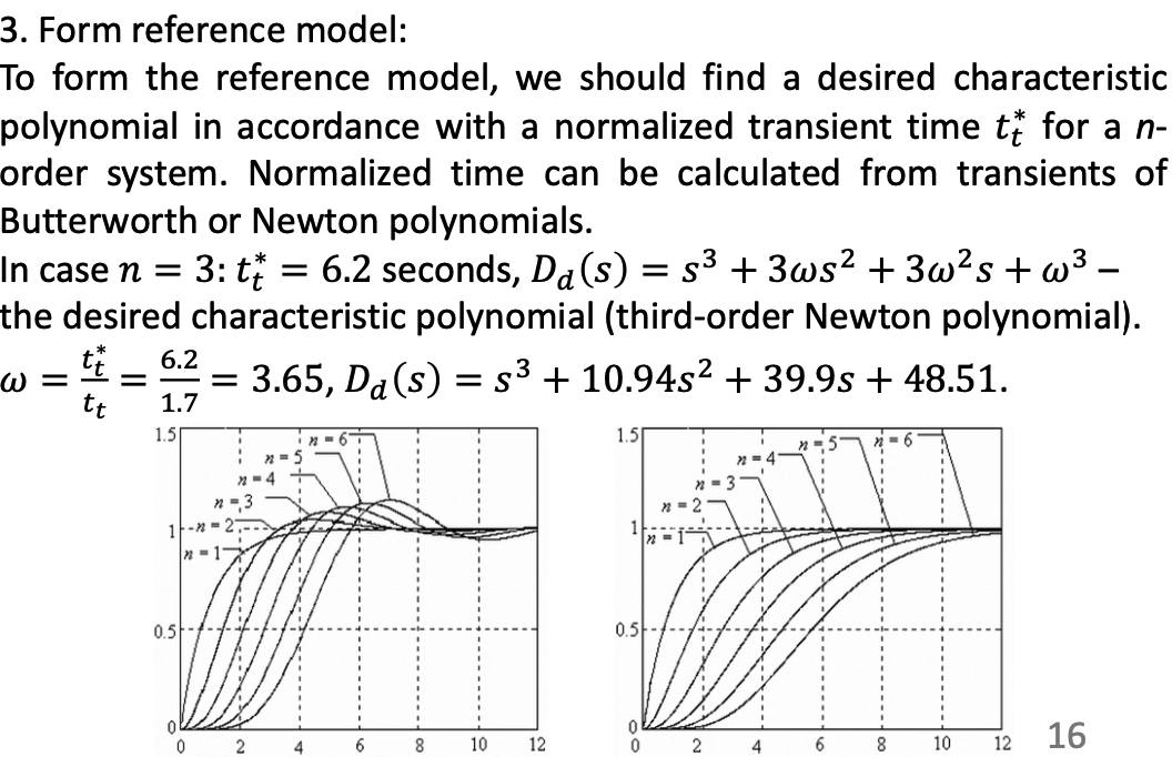
II. State Feedback design

a. Scenary

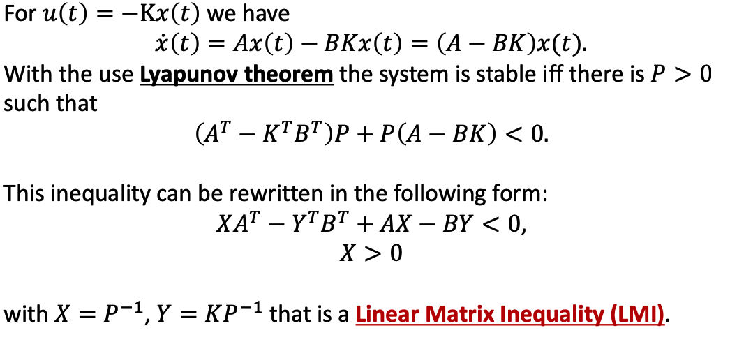
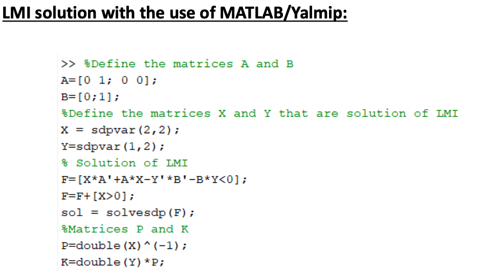
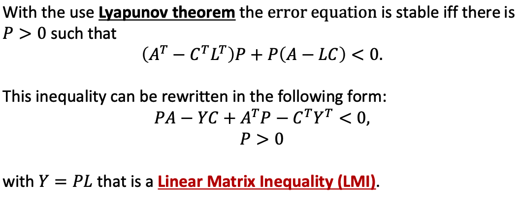
• note that the original inequality doesn’t have LMI.

b. Example

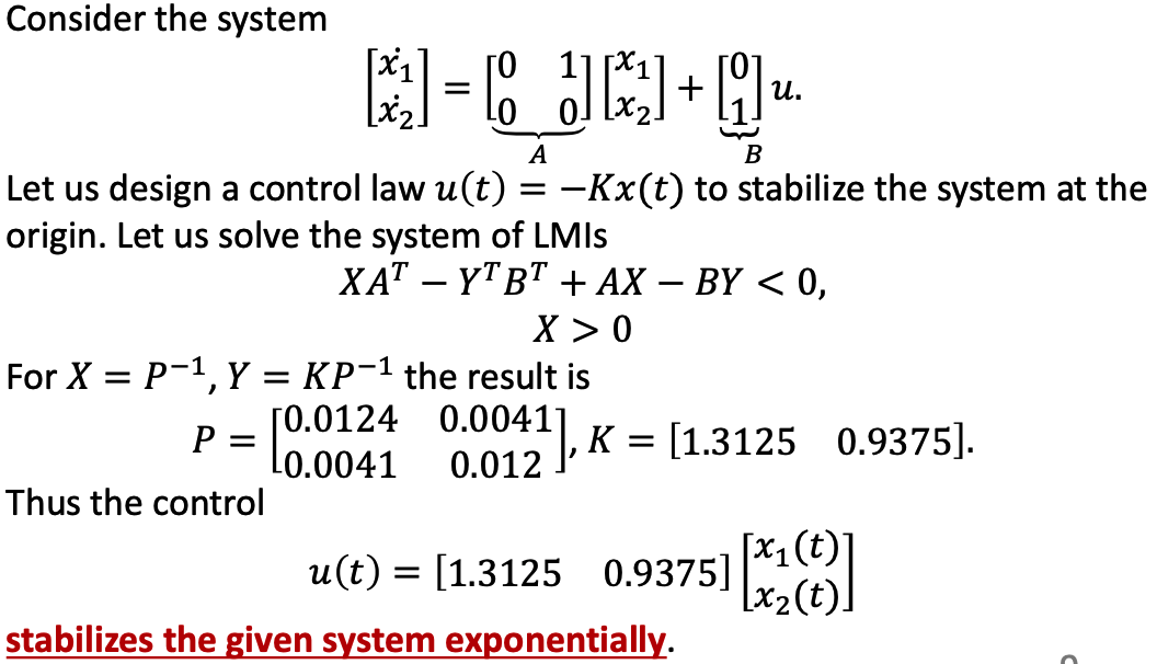
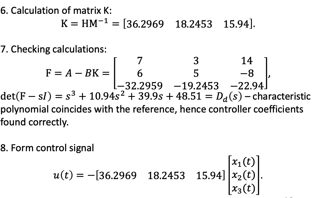
• In u(t) there should be a minus sign.

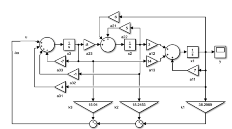
c. MATLAB realization

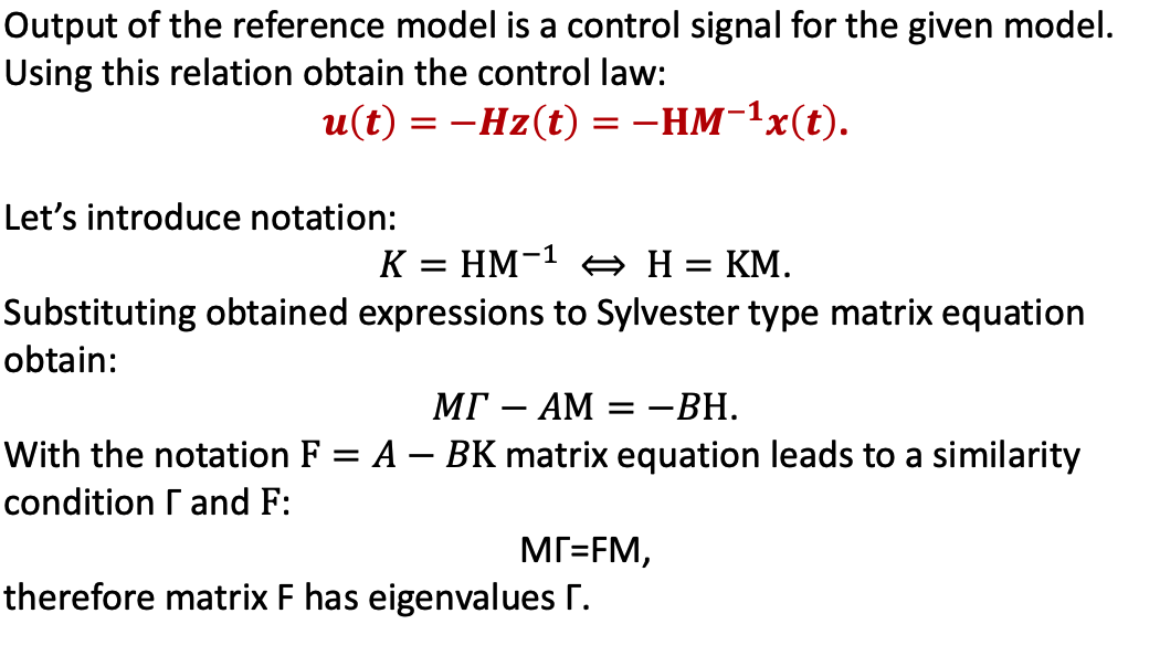
d. Modal Control

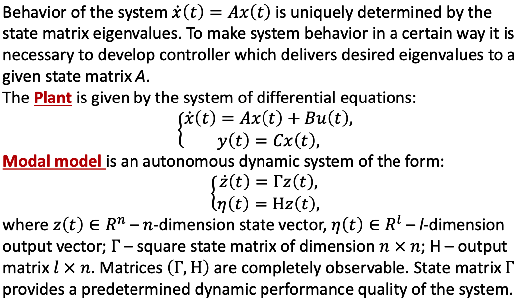
• ita and gamma in capital.

e. Example

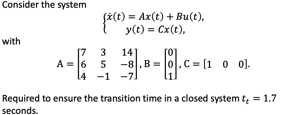
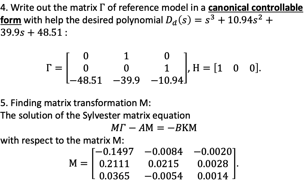
• -BKM=-BH

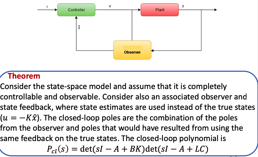
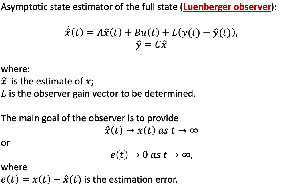
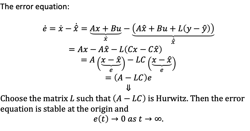
f. Observer Design

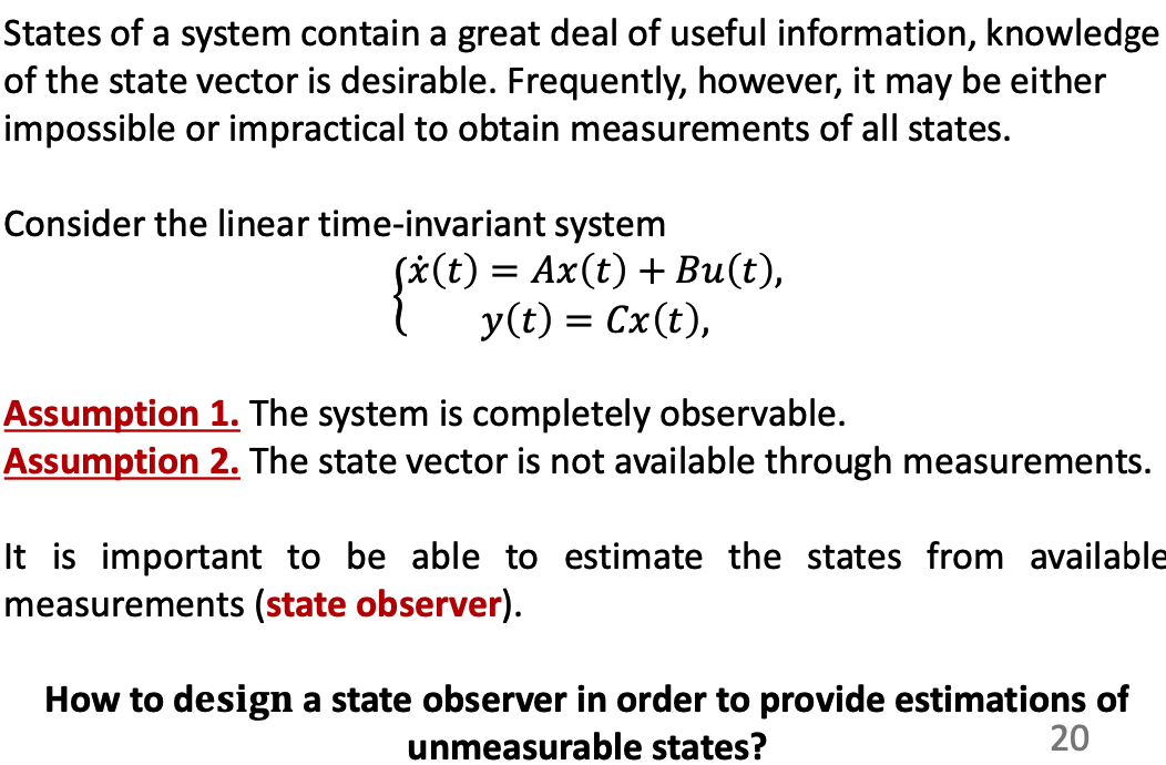
• In former lectures, we assumed that we obtain all states from output, but in practice, all states requries more moeny for sensors.
• Observer helps to see state that can’t be obtained directly.

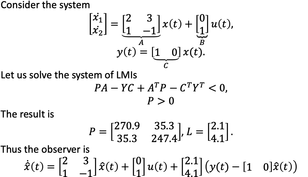
g. Example

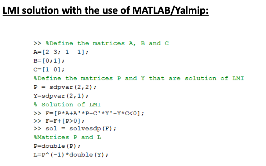
h. MATLAB realization

III. Combinition